2  Day Three Practical Q3 & Q4

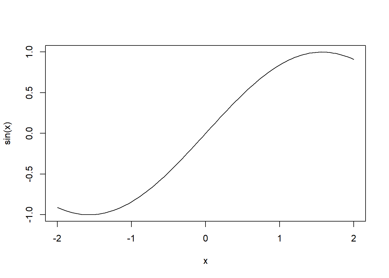
QUESTION FOUR

curve(sin(x), from = -2, to = 2) 

QUESTION FIVE

randoms <- rt(1000, 1)

#Creating a manual QQ-plot with 95% confidence interval

sorted_randoms <- sort(randoms)

n <- length(randoms)
i <- 1:n

# Calculate plotting positions (probabilities)
p <- (i - 3/8) / (n + 1/4)

# Generate normal quantiles by simulation (since we can't use qnorm)
large_normal_sample <- rnorm(1000000)  # Large normal reference
theoretical_quantiles <- quantile(large_normal_sample, probs = p)

# Calculate 95% probability envelopes by simulation
n_sim <- 1000  # Number of simulations
envelope_matrix <- matrix(NA, nrow = n_sim, ncol = n)

# Simulate many normal samples of size n
for (j in 1:n_sim) {
    sim_sample <- rnorm(n)
    sim_sorted <- sort(sim_sample)
    envelope_matrix[j, ] <- sim_sorted
}

# Calculate 2.5% and 97.5% percentiles at each position
lower_envelope <- apply(envelope_matrix, 2, quantile, probs = 0.025)
upper_envelope <- apply(envelope_matrix, 2, quantile, probs = 0.975)

# Create the QQ-plot
par(mfrow = c(1, 2))  # Split plot window

# Manual QQ-plot
plot(theoretical_quantiles, sorted_randoms,
     xlab = "Theoretical Normal Quantiles",
     ylab = "Sample Quantiles",
     main = "Manual QQ-plot with 95% Envelopes",
     pch = 19, cex = 0.6,
     ylim = c(-5, 5), xlim = c(-4, 4),
     col = rgb(0, 0, 0, 0.7))

# Add reference line (y = x)
abline(a = 0, b = 1, col = "red", lwd = 2)

# Add 95% probability bands
lines(theoretical_quantiles, lower_envelope, 
      col = "blue", lty = 2, lwd = 2)
lines(theoretical_quantiles, upper_envelope, 
      col = "blue", lty = 2, lwd = 2)

# Add legend
legend("topleft", 
       legend = c("Data", "Reference Line", "95% Envelope"),
       col = c("black", "red", "blue"),
       pch = c(19, NA, NA),
       lty = c(NA, 1, 2),
       lwd = c(NA, 2, 2))

# Check with car::qqPlot for comparison
library(car)

Loading required package: carData

qqPlot(randoms, envelope = 0.95, ylim = c(-5, 5),
       main = "car::qqPlot for Comparison",
       xlab = "Normal Quantiles",
       ylab = "Sample Quantiles")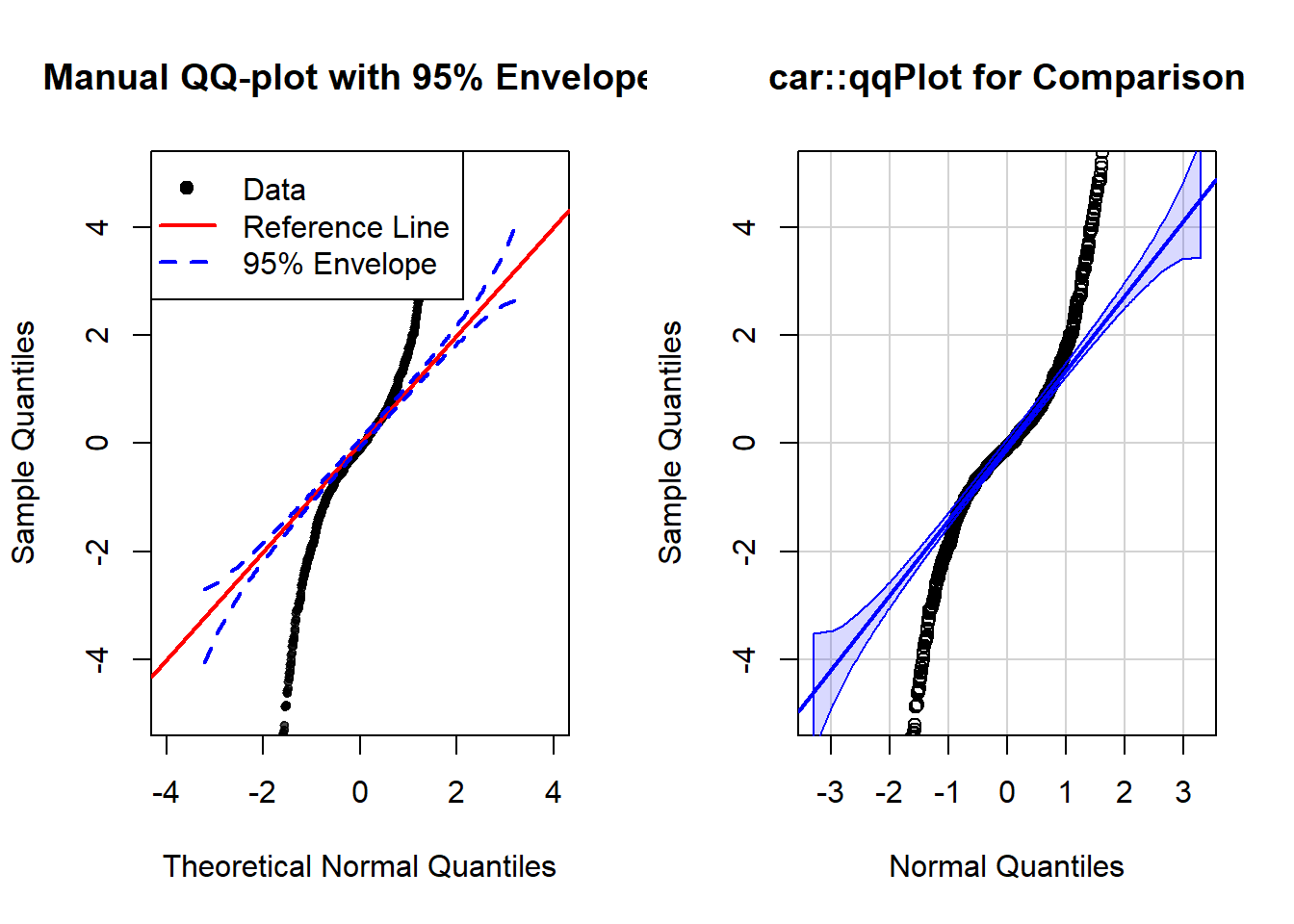

[1] 236 267